How neural network errors differ from standard code
Debugging neural networks is different from fixing standard software. In regular code, you're usually hunting a syntax error or a logical flaw. With neural networks, the problems are quieter. Training is non-deterministic, and with millions of parameters, the 'black box' nature of the model makes it hard to see where things actually broke.
The debugging needs have drastically evolved. Early neural networks were relatively simple, and errors were often traceable to obvious issues. But with the rise of deep learning, larger models, and complex architectures like transformers, we’re dealing with systems where a single error can have cascading effects that are difficult to pinpoint. It’s no longer sufficient to just check for typos; we need to understand the behavior of the network as a whole.
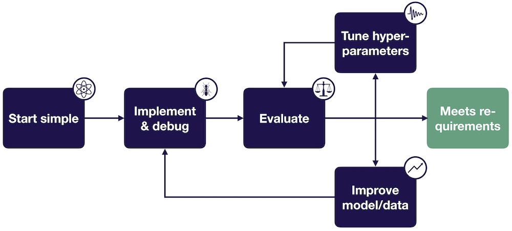
This complexity means debugging now requires a shift in mindset. It’s less about finding a single 'bug' and more about understanding why the model is making the predictions it is. This often involves looking at data, activations, gradients, and other internal states of the network. It’s about building intuition for what a healthy network looks like and identifying deviations from that norm.
The stakes are also higher. These models are increasingly used in critical applications—healthcare, finance, autonomous vehicles—where errors can have serious consequences. Therefore, robust debugging techniques are not just a matter of improving performance; they’re essential for ensuring safety and reliability.
Data is Often the Culprit
Most of the time, your model isn't the problem—your data is. I've found that cleaning and validating the dataset usually yields better results than spending a week tweaking hyperparameters. If the input is garbage, the output will be too.
Common data-related problems include missing values, incorrect labels, and inconsistencies in data formatting. Even seemingly minor errors in the dataset can have a disproportionate impact on model performance. Data distribution shifts, where the data the model sees during inference differs from the data it was trained on, are also a frequent source of problems. For example, a model trained on images taken during the day might perform poorly on images taken at night.
Data biases represent another critical issue. If the training data reflects existing societal biases, the model will likely perpetuate and even amplify those biases. This can lead to unfair or discriminatory outcomes. Thoroughly analyzing the data for potential biases is crucial before training any model.
Techniques for identifying these problems include data visualization (histograms, scatter plots, box plots) and statistical analysis (calculating summary statistics, looking for outliers). Tools like Pandas and Seaborn in Python are invaluable for these tasks. It’s also helpful to manually inspect a sample of the data to get a feel for its quality and identify any obvious errors.
- Use Pandas’ isnull() and fillna() to catch missing values.
- Verify label accuracy: Manually inspect a random sample of labeled data.
- Analyze data distributions: Use histograms and density plots to identify skewed distributions.
- Look for outliers: Use box plots and scatter plots to detect unusual data points.
Visualizing model behavior
One of the most powerful ways to understand what’s happening inside a neural network is to visualize its behavior. Activation visualization allows you to see what features individual neurons are responding to. By visualizing the activations for different inputs, you can gain insights into which parts of the network are responsible for making specific predictions.
Weight visualization can reveal patterns in the network’s weights. For example, you might notice that certain weights are consistently large or small, or that certain layers have weights that are highly correlated. This can indicate potential problems with the network’s architecture or training process. Gradient visualization helps understand how gradients flow through the network during backpropagation.
Several excellent tools facilitate these visualizations. TensorBoard, developed by Google, is a widely used tool for visualizing training metrics, model graphs, and activations. Weights & Biases is another popular option that offers more advanced features, such as experiment tracking and hyperparameter optimization. These tools allow you to track and compare different experiments, making it easier to identify the best configurations.
Beyond these general-purpose tools, libraries like `torchviz` (for PyTorch) and `keras.utils.plot_model` (for Keras) can help visualize the model architecture itself. Understanding the structure of the network is often the first step towards debugging it.
- TensorBoard is the standard for tracking training metrics and model graphs.
- Weights & Biases: Offers advanced features like experiment tracking.
- torchviz: Visualizes PyTorch model architectures.
- Keras plot_model: Visualizes Keras model architectures.
Debugging Visualizations
- Activation Maps – Visualize the output of layers to understand which parts of the input are driving the network’s decisions. 🔎
- Weight Distributions – Examine the range and spread of weights in each layer. Unexpected distributions (e.g., all zeros, very large values) can indicate problems. 📊
- Gradient Histograms – Monitor the distribution of gradients during training. Vanishing or exploding gradients are common issues revealed by these plots. 📈
- Embedding Projections – Use dimensionality reduction techniques like Principal Component Analysis (PCA) or t-distributed Stochastic Neighbor Embedding (t-SNE) to visualize high-dimensional embeddings and identify potential clustering or separation issues. 🗺️
- Confusion Matrices – For classification tasks, a confusion matrix shows the counts of true positive, true negative, false positive, and false negative predictions, highlighting where the model is making mistakes. 🧩
- Feature Importance Plots - Understand which input features have the most influence on the model's predictions. This can help identify irrelevant or problematic features. 💡
- Layer Output Magnitudes – Track the average or maximum magnitude of outputs from each layer during training. Significant drops or spikes can signal issues. 📉
Vanishing and exploding gradients
Vanishing and exploding gradients are common problems that can hinder the training of deep neural networks. Vanishing gradients occur when the gradients become increasingly small as they are backpropagated through the network, making it difficult for the earlier layers to learn. Exploding gradients, on the other hand, occur when the gradients become excessively large, leading to unstable training.
Several techniques can mitigate these issues. Weight initialization strategies, like Xavier/He initialization, help ensure that the weights are initialized in a way that prevents gradients from vanishing or exploding. Batch normalization normalizes the activations of each layer, which can help stabilize training and allow for higher learning rates.
Gradient clipping limits the magnitude of the gradients, preventing them from becoming too large. Using different activation functions, such as ReLU (Rectified Linear Unit) or LeakyReLU, can also help. ReLU, for example, avoids the vanishing gradient problem that can occur with sigmoid activation functions.
Understanding why these techniques work is crucial. Weight initialization aims to keep the variance of activations consistent across layers. Batch normalization reduces internal covariate shift, making the optimization landscape smoother. Gradient clipping prevents large updates that can destabilize training. Choosing the right activation function depends on the specific problem and network architecture.
Gradient Issue Mitigation Techniques: A Comparison
| Technique | Pros | Cons | Complexity | Typical Use Cases |
|---|---|---|---|---|
| Weight Initialization | Can prevent vanishing/exploding gradients early in training. 🚀 | Requires careful selection of initialization scheme; not a universal fix. | Low to Moderate | Deep networks, especially when starting training from scratch. |
| Batch Normalization | Accelerates training, reduces internal covariate shift, can improve generalization. 📈 | Can introduce dependencies between samples in a batch; performance can degrade with small batch sizes. | Moderate | Convolutional Neural Networks (CNNs), Recurrent Neural Networks (RNNs), and generally any deep network. |
| Gradient Clipping | Prevents exploding gradients, stabilizing training. 🛡️ | Can mask true gradient information if clipping threshold is too low; requires tuning. | Low | Recurrent Neural Networks (RNNs) where exploding gradients are common, especially with long sequences. |
| Activation Function Choice | Different activations have different gradient properties (e.g., ReLU avoids vanishing gradients for positive inputs). | Some activations can suffer from the 'dying ReLU' problem; careful selection is needed. | Low to Moderate | Varies greatly depending on network architecture and task. ReLU and its variants are common starting points. |
| Gradient Scaling | Addresses vanishing gradients by scaling gradients during backpropagation. | May require careful tuning of the scaling factor to avoid instability. | Moderate | Very deep networks or networks with specific architectural constraints. |
| Careful Learning Rate Selection | A well-tuned learning rate can prevent oscillations and ensure stable convergence. | Finding the optimal learning rate can be time-consuming and require experimentation. | Moderate | All neural network training scenarios. |
Illustrative comparison based on the article research brief. Verify current pricing, limits, and product details in the official docs before relying on it.
Overfitting and Regularization Strategies
Overfitting is a common problem where the model learns the training data too well, resulting in poor generalization to unseen data. The model essentially memorizes the training examples instead of learning the underlying patterns. This is particularly prevalent in complex models with many parameters.
The bias-variance tradeoff is central to understanding overfitting. A high-bias model is too simple and underfits the data, while a high-variance model is too complex and overfits. The goal is to find a sweet spot where the model has just enough complexity to capture the underlying patterns without memorizing the training data.
Regularization techniques help prevent overfitting by adding a penalty to the loss function that discourages complex models. L1 and L2 regularization add a penalty proportional to the absolute value or square of the weights, respectively. Dropout randomly drops out neurons during training, forcing the network to learn more robust features. Early stopping monitors the model’s performance on a validation set and stops training when the performance starts to degrade.
Regularization isn’t just about improving generalization; it also makes the training process more stable. By preventing the weights from becoming too large, regularization can help avoid the exploding gradient problem. It's a powerful tool for building models that perform well in the real world.
Tools for Automated Code Review
Automated code review tools are emerging as a valuable aid in debugging neural networks. These tools aim to identify potential errors and vulnerabilities in the code before they manifest as runtime issues. Static analysis tools examine the code without executing it, looking for things like unused variables, potential type errors, and code style violations.
Dynamic analysis tools monitor the model’s behavior during training and inference, looking for anomalies like unexpected activations or gradients. These tools can help detect issues that are difficult to find with static analysis alone. However, the field is still relatively new, and the effectiveness of these tools varies.
DeepCheck is one tool designed specifically for validating machine learning models, focusing on data quality and model correctness. Evidently AI provides tools for monitoring model performance and detecting data drift. These tools can help automate parts of the debugging process, freeing up engineers to focus on more complex issues.
These tools won't solve every problem, but they catch the obvious mistakes that usually waste an afternoon. We'll likely see more specialized tools as the tech gets better.
- DeepCheck: Validates machine learning models and data quality.
- Evidently AI: Monitors model performance and detects data drift.
- Static Analysis: Identifies potential errors without executing code.
- Dynamic Analysis: Monitors model behavior during training/inference.
Featured Products

Provides a foundational understanding of neural networks, crucial for grasping the underlying principles of the code you'll be debugging.

Essential for debugging generative AI models by ensuring that issues stem from the model itself and not from poorly constructed inputs.

Offers critical insights into monitoring and explaining AI behavior, vital for pinpointing the root causes of bugs in complex neural networks.

Addresses the unique challenges of debugging large-scale AI models, introducing SRE and chaos engineering principles for robust error detection.

While focused on web debugging, Fiddler's principles of inspecting network traffic and request/response cycles can offer valuable analogies and techniques for debugging AI model interactions and data flow.
As an Amazon Associate I earn from qualifying purchases. Prices may vary.
Debugging in Production: Monitoring and Logging
Debugging doesn’t end when the model is deployed to production. In fact, it’s arguably even more important at this stage. Production environments are often more complex and unpredictable than training environments, and issues can arise that were not apparent during development.
Monitoring model performance is crucial. Tracking metrics like accuracy, precision, recall, and F1-score can help detect when the model’s performance is degrading. Logging predictions and inputs allows you to analyze the model’s behavior in real-time and identify the root cause of any issues. Setting up alerts for anomalies can help you proactively address problems before they impact users.
Concept drift occurs when the relationship between the input features and the target variable changes over time. Data drift occurs when the distribution of the input features changes. Both can lead to a decline in model performance. Detecting these drifts requires continuous monitoring of the input data and model predictions.
A robust monitoring pipeline is essential for catching issues before they impact users. This pipeline should include data validation, performance monitoring, and anomaly detection. It should also provide mechanisms for alerting engineers when problems are detected and for rolling back to previous versions of the model if necessary.


No comments yet. Be the first to share your thoughts!